
In our previous two posts, we described how to incorporate PV diversity (diversity in both design configuration and geography) in fleet-level modeling, and how to generate high frequency fleet power data with 60-second temporal resolution. In this post, we will show how high frequency fleet data can be put to use in solving one of the key utility solar integration problems: load balancing under increased variability caused by solar PV.
The challenge of integrating variable generation
Utility grid operators (ISOs and vertically integrated utilities) are tasked with balancing the production of electrical power with its consumption. They do this by operating flexible resources to rapidly increase or decrease generation in response to changes in customer load. When high levels of variable power production from sources such as PV are introduced onto the grid, however, the problem of load balancing becomes more difficult. This is because PV production can fluctuate with cloud-transients, and the utility then has to regulate not only changes in load, but also changes in PV production.
Load balancing is performed on multiple time scales. For example, some generating resources may be dispatched on an hourly basis, some on a five-minute basis (‘real time’), and others every few seconds. The units dispatched every few seconds follow the automatic generation control (AGC) signal in order to keep system frequency in check. For purposes of this article, we are focused on one-minute to five-minute load balancing.
Quantifying the additional load balancing resources required for PV has previously required a fair amount of guesswork because high frequency, time-synchronized data from large numbers of PV systems has not been available. The approach described in this article addresses this problem by modeling PV fleets using high frequency data to produce the required datasets for planning engineers.
Estimating regulation requirements
As described in the earlier posts, PV fleet production can be simulated on a 60-second basis. This means that fleet production is available as a series of MW power values with 60-second intervals, and this series may extend over a specified study period, such as a year.
Each 60-second interval can be characterized by its change in PV fleet power. For example, if the PV production is 1,000 MW at 12:00 and 990 MW at 12:01, then there is a drop in PV power output of 10 MW. In response to this activity, the utility must increase its power production by 10 MW over the same interval to make up for the change.
Change in PV fleet power may be either positive or negative. When positive, the utility must decrease production of other resources. When negative, the utility must increase production of other resources. In either case, the goal is for the utility to produce exactly the right amount of power, given the current PV production and load.
Figure 1 illustrates a histogram of the change in power for a sample PV fleet over a year study period. The X axis shows the change in fleet power in a given interval, and the Y axis shows the number of occurrences of this change over the year. Using data in this format allows us to select a reasonable confidence interval for regulation requirements. For example, the chart shows a 99% confidence interval, meaning that 99% of the data falls within the two vertical red lines.
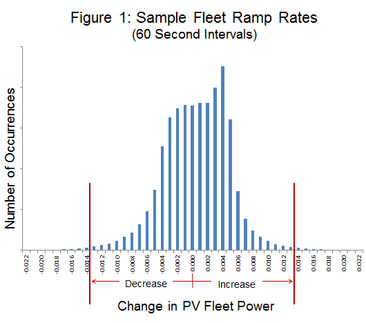
In this example, the chart indicates that at any given time, we have 99% confidence that the PV fleet will not exceed 0.013 MW of change (up or down) during any minute of the year for each MW of installed fleet capacity. For example, if the PV fleet were 1,000 MW, then at any moment we would be 99% confident that the fleet will not ramp up or down by more than 13 MW per minute.
Of course, in this example, the power fluctuations would be much less than 13 MW in the middle of clear days. These times of much lower fluctuations are quite frequent, and are represented by the observations found in the middle of the chart. But during times of patchy clouds, when PV production goes from full power to minimal power and back again, the changes in power are more significant.
Utility planners are concerned with worst case conditions, so the full year is used as a basis (a year covers the worst case seasonal patterns). In this example, the planner might decide to use the 13 MW as an extreme case, and plan the system to be able to handle ramping (up or down) of 13 MW per minute.
The example also illustrates the benefits of geographic diversity. A single small rooftop PV system may fluctuate about 90% of its maximum power output during periods of high variability. Yet, when the fleet is spread out over a large area, at least in this example, the ratio is about 1.3%.
Customizing the dataset
Using the high frequency simulation approach available with SolarAnywhere® FleetView®, utilities are able to model a variety of scenarios quickly and cost-effectively. All that is needed is the underlying high frequency weather data, available with SolarAnywhere® Data, and a clear definition of the PV resources, which are ideally obtained during the incentive or interconnection process.
With FleetView, a utility could generate a dataset similar to the one above that is based on its local conditions (available solar resource) and assumptions (size, system specifications, location of each system within the fleet, etc.). The dataset would be unique for the load balancing area in question, and for the local PV resources. For future planning, datasets could be created to look at other scenarios, such as ‘high penetration’ build-outs, or the effect of anticipated large utility-scale plants.
PV fleet modeling: Enabling better grid integration of distributed resources
In this series of blog posts, we examined some of the methods used to simulate and analyze PV fleets. While metered data from individual PV systems can be used, it is often not available at a suitable number of locations or has insufficient temporal resolution. Fleet simulation, however, puts powerful tools into the hands of utility planners and operators to help understand the impact of widespread PV on existing utility systems.
While managing the impact of PV on today’s power grid or studying future scenarios was once a major challenge, PV fleet modeling methods and tools are now available to take the uncertainty out of the equation.